ASYMPTOTIC ANALYSIS

When input sizes large enough to make only the order of growth of the running time relevant, here we are studying the asymptotic efficiency of algorithms. That is, we are concerned with how the running time of an algorithm increases with the size of the input in the limit, as the size of the input increases without bound.

Usually, an algorithm that is asymptotically more efficient will be the best choice for all but very small inputs.

Asymptotic notation, functions, and running times

We will use asymptotic notation primarily to describe the running times of algorithms, asymptotic notation actually applies to functions, the functions to which we apply asymptotic notation will usually characterize the running times of algorithms. But asymptotic notation can apply to functions that characterize some other aspect of algorithms (the amount of space they use, for example), or even to functions that have nothing whatsoever to do with algorithms.

Even when we use asymptotic notation to apply to the running time of an algorithm, we need to understand which running time we mean. Sometimes we are interested in the worst-case running time. Often, however, we wish to characterize the running time no matter what the input.

In other terms, we often wish to make a blanket statement that covers all inputs, not just the worst case. We shall see asymptotic notations that are well suited to characterizing running times no matter what the input.

Θ-notation

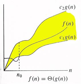
The notation Θ(n) is the formal way to express both the lower bound and the upper bound of an algorithm’s running time. For a given function g(n), we denote by Θ(g(n)) the set of functions

Θ(g(n)) = {f(n) : there exist positive constants c1, c2, and n0 such that


0≤ c1g(n)≤ f(n)≤ c2g(n) for all n≥n0 }.

Figure

Ο-notation

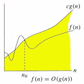
The ‚Θ-notation asymptotically bounds a function from above and below. When we have only an asymptotic upper bound, we use O notation. For a given function g(n) we denote by O(g(n)) (pronounced “big-oh of g of n” or sometimes just “oh of g of n”) the set of functions

O(g(n)) = {f(n) : there exist positive constants c and n0 such that


0≤f(n)≤cg(n) for all n≥n0 }.

We use O-notation to give an upper bound on a function, to within a constant factor.

Figure shows the intuition behind O-notation. For all values n at and to the right of n₀, the value of the function f(n) is on or below cg(n).

Ω-notation

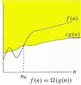
Just as O-notation provides an asymptotic upper bound on a function, $-notation provides an asymptotic lower bound. For a given function g.n/, we denote by Ω(g(n)) (pronounced “big-omega of g of n” or sometimes just “omega of g of n”) the set of functions

Ω(g(n)) ={ f(n) : there exist positive constants c and n0 such that


0≤cg(n)≤f(n) for all n≥ n0 }.

Figure shows the intuition behind $-notation. For all values n at or to the right of n₀, the value of f(n) is on or above cg(n).

Common Asymptotic Notations: Following are some common notations:

Greedy Algorithms

Algorithms for optimization problems typically go through a sequence of steps, with a set of choices at each step. For many optimization problems, using dynamic programming to determine the best choices is overkill; simpler, more efficient algorithms will do.

A greedy algorithm always makes the choice that looks best at the moment. That is, it makes a locally optimal choice in the hope that this choice will lead to a globally optimal solution. Greedy algorithms do not always yield optimal solutions, but for many problems they do. The greedy method is quite powerful and works well for a wide range of problems.

The greedy method is a general algorithm design paradigm, built on the following elements.

Configurations: different choices, collection, and values to find.

Objective function: a score assigned to configurations, which we want to either maximize or minimize

Applications of the Greedy Strategy

• Optimal Solutions:

1. change making for “normal” coin denominations
2. minimum spanning tree (MST)
3. single-source shortest paths
4. simple scheduling problems (Activity Selection)
5. Huffman codes

• Approximations/heuristics:

1. Travelling Salesman Problem
2. Knapsack Problem
3. Other Combinatorial Optimization problems